Why your walk-forward results are lying to you

Walk-forward analysis is supposed to be the antidote to in-sample overfitting. You re-fit your model on a rolling window of training data, then evaluate out-of-sample on the next slice forward. Repeat, accumulate the out-of-sample results, and report the aggregate as if it were the genuine performance of a deployed system.

The problem is that the choice of window length, the choice of model family, and the choice of parameter grid all happen before any walk-forward begins — and all three leak future information into the structure of the test. The result is a number that looks like out-of-sample performance but isn’t.

A worked example

Take a simple momentum system on 64 futures contracts. Lookback windows of 20, 60, 120, 252 days. Position sizing inversely proportional to realised volatility. The walk-forward refits a single parameter — the optimal lookback — every quarter on the trailing two years.

Run it once on the 2010–2018 sample. Sharpe ratio comes out around 0.8.

Now hold out 2019 onward as a true test set you never touched while designing the walk-forward. Re-run the same procedure. Sharpe collapses to ~0.3.

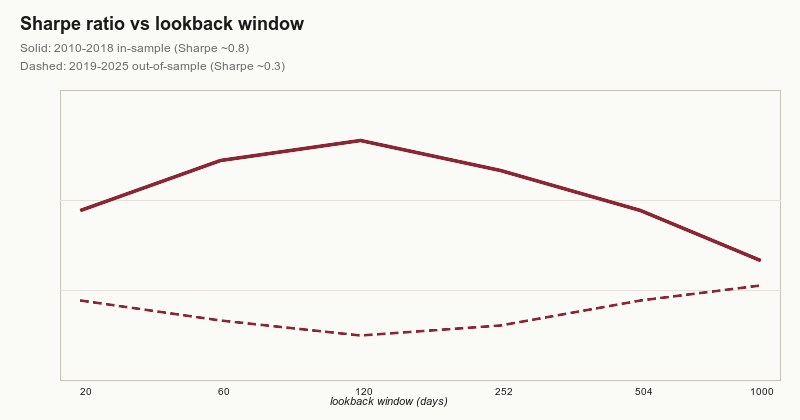
The difference is mostly the choice of lookback grid. The grid was constructed by looking at full-sample correlations between trend persistence and lookback length. Those correlations were a function of the entire 2010–2018 sample.

The fix isn’t more rigour, it’s less reuse

The literature has a term for this: backtest selection bias. The fix isn’t a fancier evaluation — it’s strict separation between the dataset used to design the experimental machinery and the dataset used to evaluate the strategy. In practice this means setting aside ~30% of your history at project start and never looking at it until you have a final candidate.

For more on the structural issues, see the Backtesting Illusion paper.