Ten things about markets that seem obvious

Every trader carries around facts about markets they don’t remember learning: that the money is made during the trading day, that weekends are dangerous, that gold goes up when stocks crash, that the London open is when gold and currencies move most, and that copper knows where stocks are heading. They come from books, from magazine articles, from forums, and from watching screens, and because they sound right, they rarely get checked.

We checked ten of them, taking the beliefs from more than 40 years of publications. The data is our archive of one-second bars, built from every trade, for 19 CME futures markets from June 2010 to October 2026. We cover the four US equity index futures, crude oil and natural gas, three metals (gold, silver, and copper), three Treasury futures, four currency futures, corn and soybeans, and bitcoin, with bitcoin and the Russell 2000 starting in 2017. Some of the ten turn out to be false, a few hold up, and others are true in a way that has nothing to do with the reason people give for them, which in trading can be just as expensive. For some of them we couldn’t find the reason at all.

1. “The money is made during the trading day”

The US session, from the cash open at 08:30 Chicago time to the futures settlement at 15:00, is where the volume is, where the news lands, and where most traders watch, yet the S&P 500 made most of its money outside it. From each day’s settlement to the next morning’s 08:30 open, the E-mini S&P 500 futures earned 8.1% a year from 2010 to 2026 (t 3.2), against 4.7% during the US session (t 1.5). The Nasdaq-100 earned 11.7% overnight and 5.3% in the session. The overnight return was positive in 15 of the 17 years for both, it was the calmer half of the day (10% annualised volatility against 13%), and it hasn’t faded: since 2018, ES made 8.7% a year overnight and 2.6% in the session.

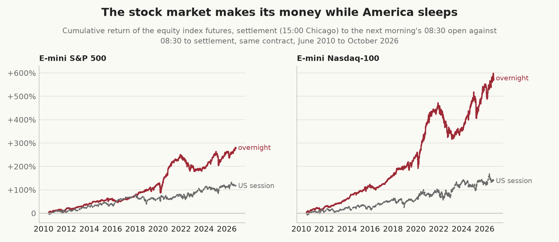
The night’s lead over the day is less certain than those figures make it look. Taken day by day, ES’s overnight return beat its session return by 3.4% a year with a t statistic of 0.9, and resampling whole months puts the difference anywhere from −3.5% to +10.3% a year (for the Nasdaq-100, 6.4%, from −1.9% to +14.9%). Over these 16 years the session earned less, so the heading is wrong about the money that was actually made, but the data can’t say which half of the day will earn more in future.

Cliff, Cooper, and Gulen documented the overnight effect in US stocks in 2008, and Bondarenko and Muravyev found it in these same futures, much of it around the European open, and our figures repeat theirs and carry them on to 2026. The best single hour in our data was 01:00 to 02:00 Chicago time, when Europe starts trading, at 2.4% a year, though we picked it after looking at all 23 hours, which makes its t statistic of 4.1 look stronger than it is. We haven’t turned any of this into a strategy, since holding only overnight means two trades a day and we haven’t counted what those would cost.

2. “Weekends are where the risk is”

“Weekends are riskier than overnight on weekdays.” (Rob Friesen, Stocks & Commodities, 2020)

Two days of news pile up while the market is shut, so traders cut positions on Friday afternoon. A weekend lasts 65 hours from Friday’s settlement to Monday’s 08:30 open, against 17.5 hours for an ordinary weeknight, and weekends are riskier, as Friesen says, but by much less than the hours suggest. Measured by standard deviation, the S&P 500 futures moved 13% more over a weekend than over a weeknight (a variance ratio of 1.27), gold 4% more, and the 10-year note and the euro slightly less. The bad weekends tell the same story: in ES the worst 5% of weekends lost 1.77% on average, against 1.53% for the worst 5% of weeknights, a ratio of 1.15 with a 95% interval from 0.89 to 1.44.

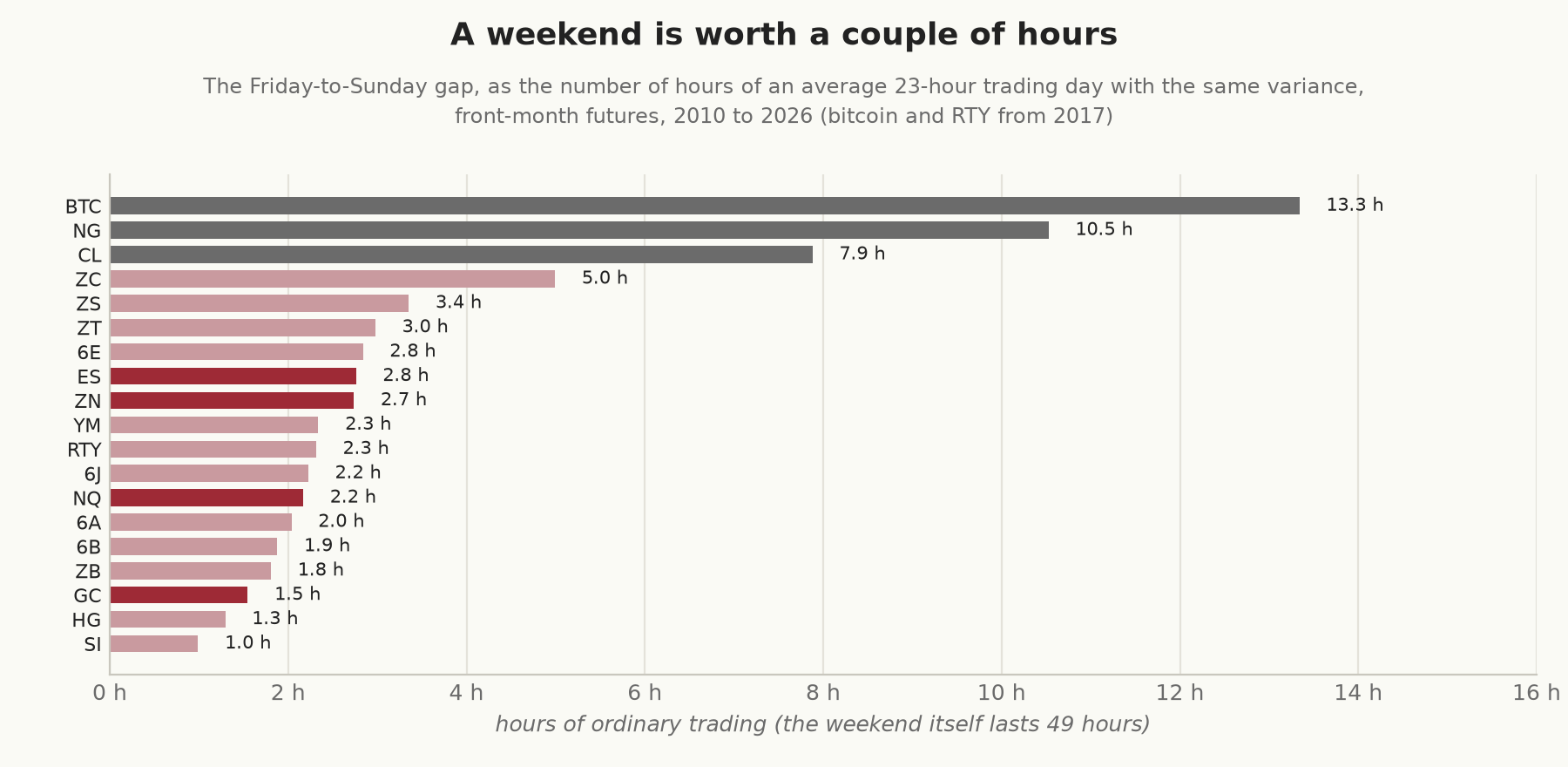
The gap itself, from Friday’s last trade to the reopening on Sunday evening, has the variance of 2.8 hours of an ordinary trading day in ES, 1.5 hours in gold, and an hour in silver, though the market is shut for 49 hours. French and Roll found the same thing in stocks in 1986: prices move because people trade on information, and over a weekend very little trading happens. The exceptions are the markets whose underlying keeps trading. Crude oil’s weekend gap has the variance of eight hours of trading, natural gas’s 10, and bitcoin’s 13, because spot bitcoin trades all weekend and the futures catch up on Sunday night. In crude the tails grow too, and its worst 5% of weekends lost 58% more than its worst weeknights (with an interval from 8% to 119% more).

These figures don’t measure what makes a weekend awkward for a trader, which is 49 hours in which a position can’t be closed at any price, followed by a Sunday reopening that may be thin. Those are reasons to cut size on a Friday even in the markets where the weekend move is barely bigger than a weeknight’s.

3. “Gold goes up when stocks crash”

“…gold remains the ultimate safe-haven asset.” (Andrea Unger, Stocks & Commodities, 2026)

On the S&P 500 futures’ worst 5% of days from 2018 to 2026, when ES fell 2.9% on average, gold fell 0.08% (with a 95% interval from −0.35% to +0.14%), and it rose on 45% of those days. In ES’s worst 1% of hours from 2010 onwards, gold fell slightly, and it rose in only 44% of them. In the first three weeks of March 2020, gold lost about 8%.

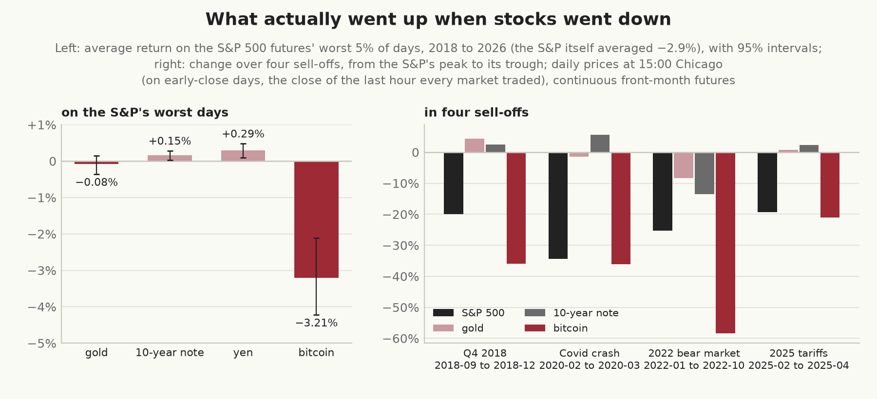
So gold didn’t go up when stocks crashed, though on average it roughly held its value. Baur and Lucey call an asset a safe haven if it’s uncorrelated with stocks, or moves against them, when stocks are falling hard, and they test that by measuring how much the asset moves with stocks on the worst days. From 2010 to 2026, gold’s slope on the S&P’s worst 5% of days was +0.02 (with an interval from −0.07 to +0.12), which is consistent with a weak safe haven, even if the interval also leaves room for gold to move a little with stocks. Since 2018 it has done just that, with a slope of +0.08 on the worst 5% of days (from +0.01 to +0.15) and +0.16 on the worst 1% (from +0.07 to +0.24). The second figure comes from only 23 days in 13 months, and a few more crises could move it a long way.

Over the four big sell-offs since 2018 gold went up twice and down twice, which isn’t something a trader can count on. The 10-year note and the yen had negative slopes on both the worst 5% and the worst 1% of days. On the S&P’s worst 5% the note rose 0.15% on average (with an interval from 0.02% to 0.28%, up on 68% of the days) and the yen 0.29% (from 0.10% to 0.48%, up on 61%).

4. “Bitcoin is a hedge”

Bitcoin was sold for years as digital gold, an asset outside the financial system that would hold its value when that system was under stress. In the CME futures it has behaved more like a volatile stock index. On the S&P’s worst 5% of days since 2018, bitcoin fell 3.2% on average (with an interval from −4.2% to −2.1%), more than the S&P’s 2.9%, and it rose on only 18% of them. In the worst 1% of S&P hours it was up 14% of the time. It fell further than the S&P in every one of the four sell-offs in the chart above: 36% against 20% in late 2018, 36% against 34% in the Covid crash, 58% against 25% in 2022, and 21% against 19% in 2025.

Its correlation with the S&P was close to zero in 2018 and 2019, then rose to 0.36 in 2020 and 0.59 in 2022, and it has been between 0.4 and 0.5 since 2024. Its beta to ES over the whole period is about one, rising to 1.2 on the S&P’s worst 5% of days, and its correlation with gold has been close to zero in most years, so it hasn’t tracked gold either.

The folklore about its weekend gaps fares no better. CME bitcoin futures are said to “always fill” the gap they leave over the weekend. Of the 428 weekend gaps since April 2018, 56% were filled within a day, against 67% for a random walk that starts at the same gap with bitcoin’s volatility over the previous 60 days, a shortfall of 10 points with an interval from 6 to 15. Over five trading days they filled about as often as the random walk would (79% against 83%), and over 20 the shortfall was three points (88% against 91%). That interval only just excludes zero, which isn’t much to go on when we looked at three horizons and the 20-day windows overlap.

5. “Bonds hedge stocks”

Much of the appeal of the 60/40 portfolio came from stocks and bonds moving in opposite directions, and for the first decade of our data they did. The correlation between daily returns of ES and the 10-year note over the previous year was below zero all the way from 2011 to 2021, and as low as −0.70 in 2012. Then inflation came back, and both fell together: in the 2022 bear market the 10-year note lost 14% while ES lost 25%. Since 2022 the correlation has moved between −0.2 and +0.4.

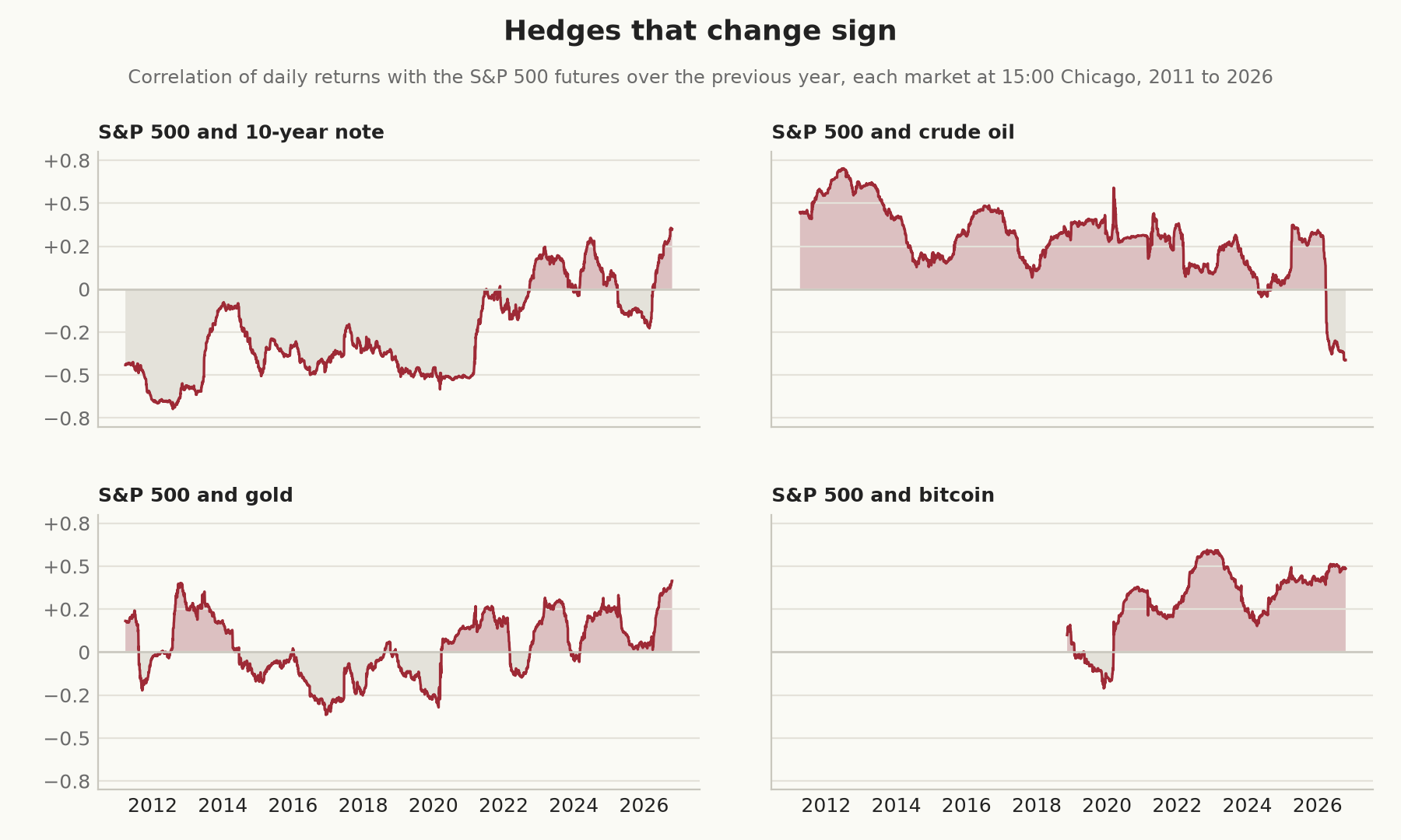
A correlation near zero, or even a modestly positive one, still spreads risk, so bonds haven’t stopped being useful in a portfolio. The trouble comes in a slow bear market, when stocks fall because rates are rising and bonds fall for the same reason. But in the sharp sell-offs they still helped, rising on two-thirds of the S&P’s worst days, and in the Covid crash the 10-year note gained 5.7%. Oil went the other way, from a correlation with stocks of +0.7 in 2012 to −0.4 in 2026.

6. “Correlation is correlation”

The correlation between two markets changes with how often you measure it. ES and NQ, two of the most closely linked markets there are, had a correlation of 0.97 day to day in 2025, 0.95 minute to minute, and 0.74 second to second. In 2012 the second-to-second figure was 0.18.

This is the Epps effect, after T. W. Epps, who described it in 1979, and it has more than one cause. In 2012 timing was probably the main one: when ES’s price changed in a given second, NQ’s changed in the same second only 27% of the time, so over a single second one had usually moved and the other hadn’t yet. By 2025 the two changed in the same second 80% of the time (90% during the US session), yet the one-second correlation was still 0.74, which suggests that most of what’s left has other causes. The likely ones (we haven’t measured how much each contributes) are the two markets' different tick sizes, a last trade that can be at the bid in one and at the ask in the other, and one market reacting a fraction of a second sooner. Across asset classes the effect is bigger and lasts longer: in 2025 the correlation of ES with the 10-year note was −0.04 at one second and −0.22 at five minutes, and with crude oil 0.09 at one second and 0.23 at five minutes.

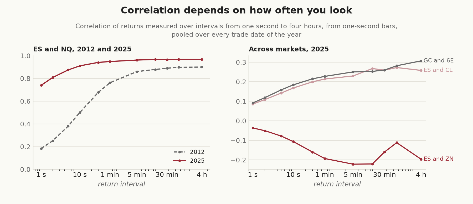
Faster markets have shrunk the effect a long way since 2012, but it hasn’t gone, and a correlation worked out directly from second-by-second trade prices still understates how closely two markets are linked. Hayashi and Yoshida’s estimator, built for prices that arrive at different moments, deals with the timing part of that without throwing the extra data away.

7. “More data gives a better measure of volatility”

If prices followed a random walk, the volatility you’d measure from one-second returns would be the same as from five-minute or daily ones, only more precise. In the 10-year note futures in 2025, the daily variance implied by one-second returns was 6.4 times the variance implied by five-minute returns, so the volatility came out 2.5 times higher. The five-minute figure isn’t the true value either, since the curve keeps falling beyond it, to about 0.7 of the five-minute variance at four hours.

The usual explanation is the bid-ask bounce: the 10-year note trades in half-32nds, a tick that’s large relative to how far it moves in a second, and trades alternate between the bid and the ask, so second by second the price jumps a tick back and forth while going nowhere. To see how much of the excess that accounts for, we took the best bid and offer in each second for a month, from 14 September to 10 October 2026. From trade prices, one-second variance in the 10-year note was 5.5 times the five-minute figure, and from the midpoint of the bid and the ask it was 3.9 times. The five-minute variance from the midpoint came out within 4% of the trade figure, so switching to the midpoint removed about a third of the excess. Most of it is still there in the midpoint, which in a market with a tick this large moves in half-tick steps as the best bid or offer is taken out and refilled, and the curve says those steps tend to reverse. ES, whose tick is small relative to its moves, was at 1.2 times from trades and 1.1 from the midpoint.

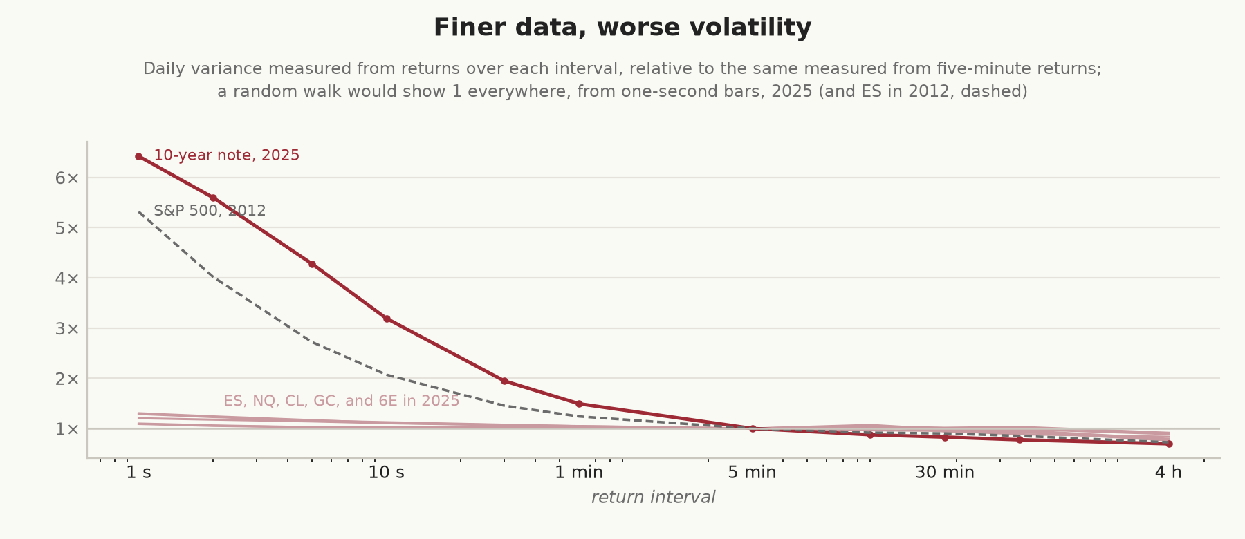
In a market with a big tick, volatility measured straight from one-second trade prices can be out by a factor of two or more, and so can any stop or position size built on it. Sampling every few minutes cuts most of the noise out in these markets, and the two-scale realised volatility of Zhang, Mykland, and Aït-Sahalia was designed to use every second despite the noise. ES itself showed 5.3 times in 2012, and by 2025, with the index four times higher and the tick still a quarter-point, it was down to 1.1 times.

8. “The London open is when gold and currencies move most”

London is the centre of the gold and currency markets, so it’s natural to expect the biggest moves of the day when London opens, at 02:00 Chicago time. In the futures, the London open shows up as only a small step. The minute with the largest average move (the largest average absolute one-minute return) in gold, the 10-year note, and the euro is 07:30 Chicago time, which is 08:30 in New York, when the US economic figures come out. The second is 09:00, when the next round of US figures does. Both fall in London’s afternoon, and London hours are still the active ones, but the biggest moves inside them come with the US figures. Even sterling’s largest average move comes at 07:30 Chicago time.

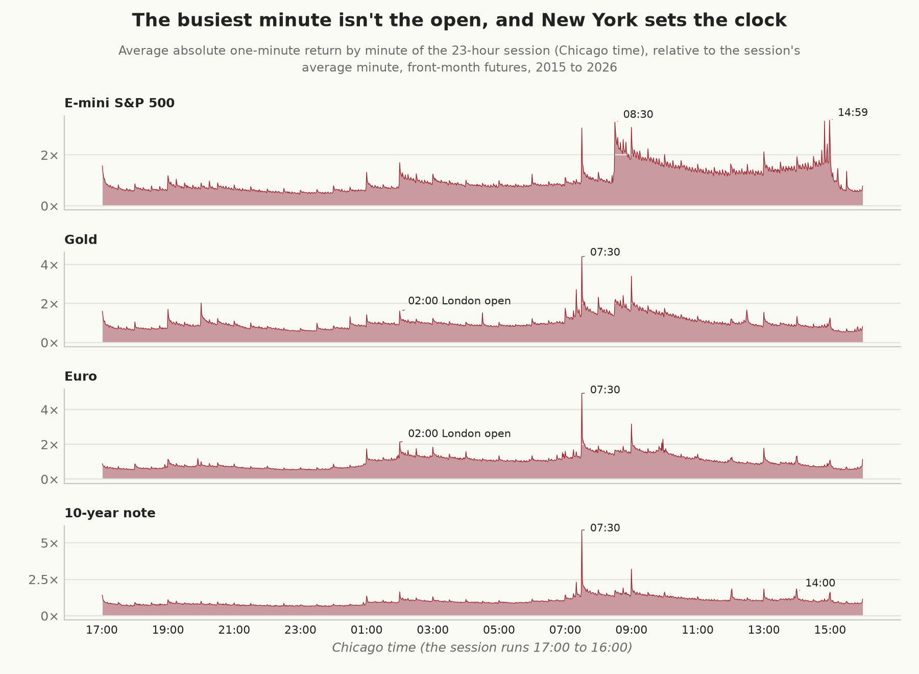
In the S&P 500 futures, Brandon Wendell’s remark that “most of the volatility comes in the morning” holds up: from 2015 to 2026 the morning, 08:30 to 11:45, had 56% of the US session’s variance, and the first hour alone had 27% of it in 15% of the minutes. But the minute with the most volume and the largest average move is 14:59 Chicago time, the minute before the daily settlement, and the 08:30 open comes third.

9. “The first hour sets the day’s high or low”

“…either the high or the low of the day is established during the first hour of trading.” (Malcolm McNutt, Stocks & Commodities, 1994)

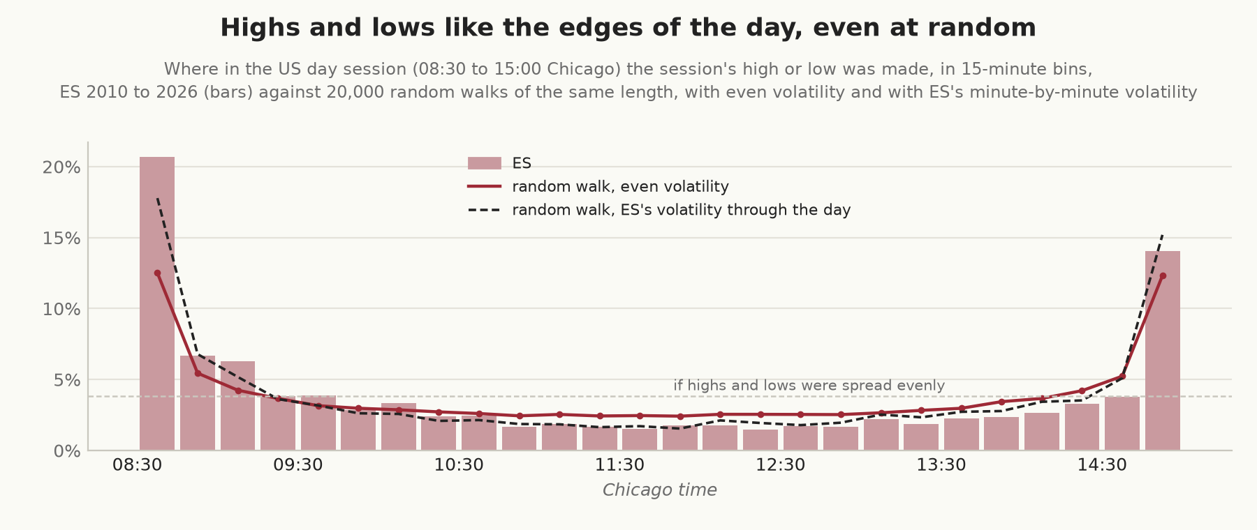
In ES’s US session, McNutt was right: on 73% of days from 2010 to 2026, the session’s high or low was made in its first hour (71% if you take the last time the high or low was touched, rather than the first). A random walk does the same on 52% of days, against the 28% you’d expect if highs and lows were spread evenly through the day.

The reason is the arcsine law: a random walk’s high is most likely to land near the start or the end of the period and least likely in the middle. A path that rises early has the rest of the day to fall away from its high, and one that rises late has had no time to come back. And the open is more volatile than the middle of the day: a random walk given ES’s own volatility, minute by minute through the session, sets its high or low in the first hour on 66% of days. That leaves five to seven points of McNutt’s figure that a random walk doesn’t produce, and we don’t know what causes them.

10. “Copper tells you where stocks are going”

“Dr Copper: Economic Health Improving Amid US-China Trade Optimism” (headline, Fawad Razaqzada, Traders.com Advantage, 2020)

Copper goes into houses, cars, power grids, and factories, so its price is supposed to turn before the economy does, which is why it’s said to have a PhD in economics. Headlines like Razaqzada’s read it as a gauge of the economy, and traders take the idea a step further and watch it for clues about where stocks are heading, which is the version we can test with prices. Copper and the S&P 500 futures do move together, with a correlation of 0.36 over the same week or month and 0.46 over the same quarter. But there’s little sign that copper moves first. The correlation between copper’s return over one period and the S&P’s over the next was −0.04 a week ahead (with an interval from −0.11 to +0.03), −0.09 a month ahead (from −0.22 to +0.05), and −0.08 a quarter ahead.

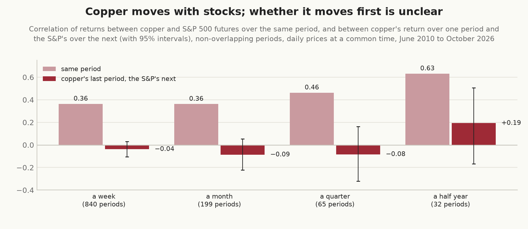
After a month in which copper rose, the S&P gained 0.96% the next month, and after a month in which it fell, 1.05%. The S&P’s past return didn’t predict copper’s either. The one positive figure, +0.19 over half a year, comes from 32 periods, and its interval runs from −0.17 to +0.51, which leaves room for anything from a small negative relationship to a fairly strong lead. The original form of the saying, that copper anticipates the economy, is a different claim, and this doesn’t test it. Stock prices may move on economic news before the figures are published, so copper could lead the economy without leading stocks, and checking that needs economic data, with allowance for publication lags and revisions.

What didn’t make the list

We tested more than these ten, and the rest held up, came out mixed, or were too close to call. When price takes out the previous day’s high or low, it goes on a tenth of a typical day’s range before coming back the same distance on 49% to 53% of occasions across six markets. That’s a coin toss for direction, though whether a breakout or a fade would make money depends on the size of the moves, the exits, and the costs, which we didn’t test.

Monday hasn’t been a bad day for the equity index futures, whose average Monday return was positive in all four (with t statistics from 1.0 to 2.5), and across all 19 markets the Monday figures were spread about as widely as chance would put them. Gaps in ES fill about as often as a random walk says they should (on 60% of days against 62%). The 10-year note’s return in one minute had a correlation of 0.005 with the S&P’s in the next. That shows up over nearly three million minutes, but it explains almost none of the variance in the S&P’s next-minute return (an R² of 0.0025%), and we haven’t tested whether anything could be traded on it.

Method notes

The futures data is the front-month contract on each CME trade date, as one-second bars built from every trade. The front month is the contract with the most volume that day, which is fine for describing the market, though a trading rule would have to choose it from what was known beforehand. A bar is dropped if its last price is further from the median of the 21 bars around it than 15% of a typical day’s range, or eight ticks if that’s larger. That removes isolated prints and keeps any move that lasts more than about ten bars, since such a move carries the median with it. A real move that reverses within a few seconds could be cut, and in ES the rule dropped between none and 16 bars a year out of 7 to 11 million. Trade dates run from 17:00 to 16:00 Chicago time, and returns that would cross a contract roll are left out.

Daily returns compared across markets (items 3, 4, 5, and 10) use every market’s price at the same time each day, whatever its own settlement time (gold settles at 12:30 and Treasuries at 14:00). That’s 15:00 Chicago time, or, on the 149 days when a market closed early, the close of the last hour that every market traded in full, and returns run between dates on which all the markets being compared have a price. The worst days, the sell-offs, and the copper test use continuous front-month series, ratio-adjusted at each roll. Each sell-off runs from the S&P’s highest daily price to its lowest: 20 September to 24 December 2018, 17 February to 23 March 2020, 3 January to 12 October 2022, and 19 February to 8 April 2025.

The safe-haven test follows Baur and Lucey: each market’s daily return is regressed on the S&P’s with an extra slope for the S&P’s worst 5% of days (or, in a separate regression, its worst 1%). The slope we report is the sum of the two, which is the whole slope on those days. Intervals for these slopes, and for averages and shares over days, come from resampling whole calendar months, since bad days cluster (for the slopes, the thresholds are re-estimated each time). Intervals for the copper correlations use Fisher’s transformation; the t statistics treat days as independent. The weekend tails compare the move from Friday’s settlement to Monday’s 08:30 open with the same span on a weeknight.

Correlations and volatility by interval (items 6 and 7) come from every trading day of 2012 and 2025, with each market’s last price carried forward on a common one-second grid, and the midpoint check uses Databento’s one-second best bid and offer. The random walks use Gaussian steps. The gap benchmarks are the chance that a random walk starting at each actual gap, with the previous 60 days' volatility, trades back to the earlier price within the window, and gaps whose window runs past the end of the data are left out of that window’s figures. Nothing here has been turned into a trading rule, and none of the results include costs.

References

• Baur, D. G., and Lucey, B. M., “Is Gold a Hedge or a Safe Haven? An Analysis of Stocks, Bonds and Gold”, Financial Review 45, 2010.
• Bondarenko, O., and Muravyev, D., “Market Return Around the Clock: A Puzzle”, Journal of Financial and Quantitative Analysis, 2023.
• Cliff, M., Cooper, M. J., and Gulen, H., “Return Differences between Trading and Non-Trading Hours: Like Night and Day”, working paper, 2008.
• Epps, T. W., “Comovements in Stock Prices in the Very Short Run”, Journal of the American Statistical Association 74, 1979.
• French, K. R., and Roll, R., “Stock Return Variances: The Arrival of Information and the Reaction of Traders”, Journal of Financial Economics 17, 1986.
• Hayashi, T., and Yoshida, N., “On Covariance Estimation of Non-Synchronously Observed Diffusion Processes”, Bernoulli 11, 2005.
• Zhang, L., Mykland, P. A., and Aït-Sahalia, Y., “A Tale of Two Time Scales: Determining Integrated Volatility With Noisy High-Frequency Data”, Journal of the American Statistical Association 100, 2005.
• Razaqzada, F., “Dr Copper: Economic Health Improving Amid US-China Trade Optimism”, Traders.com Advantage, 2020 (listed in Technical Analysis of Stocks & Commodities, bonus issue 2021).
• Friesen, R., “Trading Perspectives”, Technical Analysis of Stocks & Commodities, February 2020.
• McNutt, M., “First-Hour Breakout System”, Technical Analysis of Stocks & Commodities, July 1994.
• Unger, A., “Trend-Following Systems Under Extreme Conditions: The Gold Rally Case Study (2024–2026)”, Technical Analysis of Stocks & Commodities, August 2026.
• “Brandon Wendell And Trading Around The World”, interview, Technical Analysis of Stocks & Commodities, December 2010.